Sand Frac Mining in Wisconsin: Data Gathering and Geocoding

Introduction

The first step in the geographic inquire process is to ask a geographic question. This step was covered in the last report, where it was possible to understand the issues related to sand mining in western Wisconsin. Then, the study of the level of impact that the transportation of sands have on the roads will be done by the use of network analysis.

However, any kind of analysis will need to have data to be based on, which consist in the second step of the geographic inquire process. Then, this report will cover the procedures related to the obtainment of geographic data within the area of interest. One of the main necessary data is the location of the sand mines, which were found in a table with addresses. So, this phase does not only include the simple download of data, but also the necessary preparation of the data to be ready for the analysis. Then, the geocoding process will also be reported. Then, it’s aimed as a result to have a geodatabase containing all the necessary data adapted already for the purposes of this project.

Methodology

Firstly, a number of sources were explored: the National Atlas, the National Wetlands Inventory, the USGS National Map Viewer, the Multi-Resolution Land Characteristics Consortium (MRLC) and the U.S. Department of Agriculture (both Geospatial Data Gateway and the Soil Survey Geographic Database). Each website has a particular way to download data and different levels of availability. Since that in this particular exercise of gathering the data, the focus was in Trempealeau County, some data was downloaded for the whole state, but it was preferred to obtain the county data – usually more detailed.

After obtaining the data, it was necessary to review it to guarantee its consistency. In the case of elevation model (DEM), obtained by MRLC, there was two tiles, so it was necessary to use a mosaic tool to join this data in one only file. In one case – for the National Wetlands Inventory – the data was just not available for Wisconsin, so no data was downloaded. In other case, for the soil data, obtained by SSURGO, it was necessary to take in consideration the drainage index of each feature, so the examination of the database over Microsoft Access and the use of the join tool were necessary.

Next, the design of a geodatabase included to re-project all features to the same coordinate system. The choice is related to the available coordinate system covering the smaller area beyond the Area of Interest. Trempealeau County is located in the Central Zone for the Wisconsin State Plane System, so this was the best choice found. Then, the features were combined in a single geodatabase: Railroads (The National Atlas), Soils (SSURGO), Cropland (Geospatial Data Gateway), Land Cover (USGS) and Elevation (MRLC).

Subsequently, although all these elements are important, the crucial element for the project consists in the location of the mines. For the Trempealeau County, a geodatabase containing it was already obtained; however, since the analysis is for Western Wisconsin, and not only one county, it’s necessary to have a feature class with all the mines.

The data obtained for that consisted in a non-spatial table, where one of the fields contained its addresses and the other fields contained further information about each mine. However, the later network analysis requires a spatial feature for the mines, not only a stand-alone table.

As follows, plotting the points in the map accordingly with its addresses is necessary, which can be done by using the geocoding tool. Geocoding, as said, consists in giving X,Y locations for entities using their address field. It’s based in a locator that has the settings related to the specifications of the type of address used; the necessary fields and, mainly, relies on a reference feature. This can consist in a line feature for the roads, which will use the nodes to find a precise place for the number address. It can also consist in polygons, where the address will be based on zip or state, and the point will be located in the centroid of the polygon. Points are an option for the reference data as well, and would be the most precise scenario, because the output would match the point address of the reference feature. After having the locator, it’s necessary to have a normalized table that fits the specific requirements of the locator used.

For this exercise, the locator chosen was “TA_Address_NA”, which used to be provided by ESRI. In the new version of ArcGIS, the locator is still accessible, but it’s necessary to connect to a specific server. In the near future, it’s possible that this locator might have a restricted access. Anyhow, this locator uses address, city, state and zip fields. The table obtained, however, didn’t have these divisions. Then, the normalization of the table was made.

Since this task is time-consuming and requires attention to the detail, the class was divided in groups of four people, so the division of tasks could increase the productivity. There were approximately 100 entities in the table, after excluding the ones located in Trempealeau County. Then, each person was responsible for the normalization and localization of about 25 mines.

By examining the table, it was possible to notice that the Facility Address field didn’t contain only its address, although its name. There were three types of information there: full address, containing number, street, street type, city and zip; directions, where an intersection was mentioned or a sentence with the explanation of where the place is located; and for last, the PLSS information for the mine.

Considering that, the entities were divided in three different sheets using Microsoft Excel (Figure 1): 14 entities contained full address and were supposed to correctly geocode; 4 entities were based on directions; for last, 7 entities were based on PLSS code.

Figure 1 – Division of entities in different sheets.

With that, only the “(SupposeTo)GeocodeMines” sheet needed to fit the fields of the locator, since the others would need other methods to get a X,Y location. Then, a rough division of fields was made, without much concern to abbreviations on the address, and then the geocoding tool was applied to check what might be changed. Then, the fields were adapted to match better the reference feature. For example, one of the mines had the address “S1678 CTH U”. (Figure 2). Although it’s possible to determine that S stands for South and 1678 is the number address, if you’re not familiar with the typical abbreviations, the “CTH” doesn’t have a intuitive meaning.

Figure 2 – Abbreviation in entity address.

A quick research was made to identify its meaning, resulting in “County Trunk Highway”, which is a nomination exclusive for Wisconsin. After examining the streets of the different counties by Google Earth, it was possible to understand better its structure. It’s extremely common to have different streets named simply “County Road”, which can also be referred with the county name. Inside Eau Claire County, for example, it can also be called “Eau Claire Road”. In counties less urbanized, this is the base of the street naming, using letters of the alphabet as a suffix to differentiate them. They are also usually abbreviated to “Co Rd”, which was found in other entities as well and was not easily comprehended at first (Figure 3).

Figure 3 – Structure of roads near Montana, WI

Then, after analyzing all the addresses and its possible correspondents, a new correct sheet was used to run the geocode tool with. While geocoding, it’s necessary to pay attention on the method used. The locator used will place the feature in the centroid of the zip-code, city or state in case it doesn’t fit in any other category. Then, after running the geocoding tool, it was necessary to analyze the “Loc_name” field to see to which locator the feature was matched to, the desired ones were “US_RoofTop” or “US_Streets” (Figure 4). Because the ones with “US_CityState” and “US_Zipcode” had the feature in the centroid of the polygon, they need to be manually found.

Figure 4 – Examination of “Loc_name” field to recognize unacceptable geocoding.

By comparing the current results in Arc Map to the address search using Google Earth, it was possible to manually locate the mines. A two-screen set was extremely helpful to maintain both softwares open and visible. With that, it was easier to compare ground features and locate them correctly. The ideal scenario was to find the exact location of the mines, what was possible by using some 2013 updated Google Earth satellite images available (Figure 5).

Although remote sensing is not the focus of this project, it’s important to use its skills to recognize a mine by its exclusive tone, association with buildings and trucks, which creates a peculiar circular shape. Also, with remote sensing identification skills, the comparison between the features around the mine enables its placement in Arc Map, where the image was not as updated.

Figure 5 – Typical characteristics of a sand mine using tone, shape and association.

However, not all the mines could be extremely precisely located. Not all mines listed are already built, some are not in a stage where recognition is possible and not all the satellite images are updated enough for the identification. Then, when it was not possible to visualize it, the location was based in the road or directions given by the “Facility Address” field.

This process was used for the entities not geocoded and also the ones based on directions. The difference between them is that for the first ones, an editor session was enough to change its location; while for the second ones, it was necessary to create a field on Excel to input its GCS coordinates available in Google Earth. To increase precision, it’s important to remember to use about six decimal places for GCS coordinates, since in this location, 0.1° represents approximately 8km. After the input, it was necessary to import the stand-alone table, display it using X,Y coordinates and then export the data as a feature class to the geodatabase being used.

For last, the localization of features based on its PLSS was made. It was noticed that the code was no standardized; some features had the name of the township, instead of its number and range. To be able to fix the table with the correct code, a resource provided by the Wisconsin Cartographer’s Office was used: the PLSS Finder. With that, it was possible to localize the Township and Range based on the name given, using the search tool (Figure 6). For that, it was useful to remove the PLSS Covers, some other layers such as County lines and names were useful to localize the features.

Figure 6 – Use of PLSS Finder to identify township and range numbers by its name.

After having an appropriate table, two polygon feature classes were used to localize the same locations inside Arc Map: Sections and Quarter-Sections. However, since most of features didn’t have the quarter-section information, the sections feature was essentially used. In this feature, three fields were mainly used: township (“TWP”), range (“RNG”) and section (“SEC”). 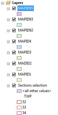The symbolization based on the township field was used to understand better the divisions of the PLSS (Figure 7). First, a query was used to select only the townships necessary and minimize the overloading of the system – which was slowing the process by then. Then, the selection was used to create a new layer, this layer was then symbolized with the townships 32, 33 and 34.

Figure 7 – Symbolization of townships in Wisconsin.

It would be possible to localize each section by the use of symbolization, but that would be time-consuming, especially with the amount of data displayed overloading the system. As faster and easier way to do that is by running a query (Figure 8). That way, the software would automatically find the features that meet the codes of the non-spatial table. The ideal would be to have only one result out of the query, but some entities were located in more than one section or range. In this cases, it was necessary to use the operator “OR” as well and the results were multiple.

Figure 8 – Use of SQL expression in the query to find the appropriate PLSS sections.

However, not only these cases had multiple results. The reason for that is on the “DIR” field. It states if the feature is in the west or east side. However, it was being represented by 2 and 4 and a legend wasn’t available. Then, the multiple results were kept and map visualization would show which direction each one had. After running each query, the selection would be used to create a new feature layer (Figure 9). Multiple layers would be helpful to keep the organization and not overload the system with a large amount of unnecessary data.

Figure 9 – Different layers to maintain organization.

Then, all the layers would be turned off and, individually, each entity would be located with an imagery base map. Then, with Google Earth open in a different screen, it would be possible to find the mine or approximate to the main street inside the section. The procedure would be similar to the ones for the directions: comparison between different satellite images, input of GCS coordinates in six decimal places, importation in ArcGIS using X,Y coordinates and later data exportation as a feature class.

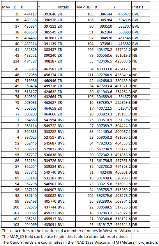
For last, with all the mines located – even if in different levels of precision – it was necessary to put all together in one only table. However, the fields were already modified and wouldn’t match. Then, a simplified table was created with the key-field “MAPID”, its coordinates and the initials of who found that location. For the coordinate fields, it was necessary to use the “Add X,Y coordinates”. All the features were kept in a geodatabase (Figure 10), so they were all projected in the same coordinate system: Wisconsin State Plane System – Central Zone (NAD 1983). For that reason, the fields created would match each other afterwards. For last, the group agreed in having the coordinates in this same coordinate system and a excel table was made with all the entities. The table would be then be imported to ArcGIS using the X,Y coordinates and later exported as a feature class.

Figure 10 - Geodatabase for the mine location finding.

Results

Therefore, the data gathering resulted in a geodatabase containing the different elements obtained (Figure 11).

Figure 11 – Geodatabase designed for data gathering.

The railroads feature class contains data for the whole United States (Figure 12), but it will be clipped to the area of interest, as soon as this area is defined.

Figure 12 – Railroads

The same generalization happens with the cropland data layer (Figure 13), obtained for the whole state of Wisconsin. In this case, it will be necessary to use a different kind of clipping tool, since it’s a raster feature.

Figure 13 – Cropland Data Layer

Then, since the exercise was focused in the Trempealeau County, some features were collected only within its area, like the soils feature class (Figure 14). The DEM mosaic (Figure 15) and the land cover feature class by NLCD (Figure 16) don’t match the exact boundary of the county, but also don’t cover much beyond that.

Figure 14 – Trempealeau County Soils Feature Class

Figure 15 – Elevation based on a DEM mosaic

Figure 16 – Land Cover by NLCD

Later on, to find the location of mines, after the division of 25 entities for each person, 14 were used in the geocoding tool, having the result of one feature tied – which was easily untied afterwards – and 13 matched. However, from those 13 matched, only seven consisted on the address locator; five of them were matched to the centroid of its zip code and one to the centroid of the city. For these six misplaced entities, the editor tool was used to replace them in the right location. Besides the ones related to the geocoding process, four entities were based in directions and seven in the PLSS code.

Considering all the entities, after joining with the rest of the group, 74 were matched (manually or by geocoding) and 25 didn’t have information enough to be matched. The result was a feature class containing the mine features, originated from Trempealeau database, plus these 74 features localized (Figure 17), based on the excel table designed (Figure 18).

Figure 17 - Sand Mines in Wisconsin

Figure 18 - Simplified table to create sand mines feature class.

Conclusion

The process of gathering data and locating non-spatial table – either manually or through the geocoding tool – is crucial for any project being made that depends on searching data and not finding only spatial files. It’s literally impossible to start your project without these steps, and the results will be the base of all the other steps, so it’s necessary to be really careful with the procedures taken. For that reason and even just because of the nature of the process, it gets time-demanding and complicated to deal with, so patience is extremely desired to deal with it.

The overload of the system is common when dealing with large datasets, especially in the data gathering, where most of the features were rasters; and if not, they contained way too much information, which made the software crash for some times.  A lot of time was also taken by the system overloads when geocoding and using satellite images in Arc Map. For that, it was very useful to use Google Earth, since it has a better performance when dragging, zooming in and out on the map.

Flexibility is also an important element for these tasks, because you frequently need to find different ways to come to an answer, such as dealing with unfamiliar abbreviations or dealing with the overload in the system.

Finally, the exercise can be considered successful in establishing the base data to be later manipulated in order to accomplish the bigger goal of the project. With the data formatted and organized as it’s after this, it will be possible to easily manage it and apply the procedures for the next steps.

Sand Frac Mining in Wisconsin: Overview

Nowadays, the lack of energy resources is one of the main worldwide issues. The main problem is that the primary source used is based on fossil fuels, which are a finite. In the recent decades, the idea of sustainability has arisen, where not only energy, but all the natural resources would need to be managed in a way to be available not only for the current generation, but for the following ones. With that, methods to obtain energy from infinite resources – such as water, wind, sunlight – has become more attractive. However, the main leaders in the world still focus their attention in the use of fossil fuels.

In this scenario, the petroleum industry keeps with its huge power over different kinds of industries. Sand mining is an old activity that serves to many purposes, such as glass production, foundry molds and a number of other uses that kept the industry alive along all these years. However, the development of a technique to extract more oil and gas using a specific kind of sand made this industry to expand increasingly again over the past years.

The process of hydraulic fracturing allows the extraction of more oil and gas from wells where it was considered unproductive already. The gas and oil is hold within a rock, and its lack of porosity can minimize the amount of product able to be explored. The method uses frac sand, water and chemicals that are injected at the rock in an extremely high pressure. The friction creates fractures in the rock and the sand guarantees the fractures will keep open. (Wisconsin DNR, 2012) With that, the porosity increases, allowing the exploration of oil and gas in a much higher rate than before.

However, not any sand can be used for this process. Firstly, to be able to cause a fracture, the composition of the rock needs to have a high level of hardness. In this case, the ideal element would be silica, commonly called quartz, which has a hardness of 7 in the Mohs scale (Figure 1). Thus, the sand extracted needs to have a high purity in this specific element. Moreover, the sand grain needs to have a specific size, which will depend on the type of deposition that formed the geological unit: if the transportation occurred in a high energy environment, the grains will be larger than if it happened in low energy transportation. Lastly, the form of the grain is also important, it needs to be very well rounded, which will also depend on the type of deposition: the longer the time of transportation, the more rounded the grains will be.

Figure 1 - Mohs Scale

In Wisconsin, a sandstone formation covers the western region and meets all these requirements mentioned. Even though another areas of Wisconsin also have potential to sand mining, they are originated from recent glaciations and beach formations, then, it’s a really impure kind of sand and also angular, instead of rounded, reason why is not appropriate for the process. (Wisconsin Geological and Natural History Survey, 2013)

Because of that, in the past years, a lot of sand mines were placed in this location. The development is happening in a high rate, reason why the department of natural resources is trying to keep track of it by encouraging a specific registration for frac sand mining in Wisconsin. Also, the authorities are concerned with the implication in the environment related to the pollution and contamination of air and water in the areas where the sand exploration is being done. In the other hand, the economic development derived from these mines appears as a benefit.

Considering this whole scenario, the analysis of the sand mines distribution and impact can be done in a lot of ways by the use of a geographic information system. For that, the geography inquiry process is used. There are a lot of specific questions that can be made about this issue because it’s very broad. Then, first is necessary to decide which part of the problem is going to be analyzed. Then, to acquire the data may be a challenging step, but extremely necessary to have consistent results. In this step, it’s necessary to keep track of the data quality, thinking of the different dimensions of accuracy. After having the appropriate data available and ready to be used, a preliminary exploration using symbolization and cartography is useful to have a basic idea of the scenario. Then, with the use of geoprocessing tools, a higher level of understanding in resulted. With that, it’s possible to provide information enough so the authorities can act in geographic knowledge.

In this project, the impact of the relation of the sand mine with its costumers – the ones who will apply the sand to the fracking process – will be the main subject. The transportation of sand involves the use of specific sorts of trucks, who carry a higher weight that the road might support. Since the roads were not built with the focus on this recent development of sand extraction, they might not be prepared for that. Then, the impact will be examined by a network analysis. As a result, it’s expected to acquire helpful information that can suggest appropriate initiatives and position from the government.

References

DEPARTMENT OF AGRICULTURE, CONSERVATION AND FORESTRY. (2005) testing the hardness of common minerals. Available: http://www.maine.gov/doc/nrimc/mgs/education/lessons/act20.htm [11 Mar 2013]

Wisconsin Department of Natural Resources (2012) Silica Sand Mining in Wisconsin [Online], Available: http://dnr.wi.gov/topic/Mines/documents/SilicaSandMiningFinal.pdf  [11 Mar 2013]

Wisconsin GEOLOGICAL AND NATURAL HISTORY SURVEY (2013) Frac Sand in Wisconsin [Online], Available: http://wisconsingeologicalsurvey.org/pdfs/frac-sand-factsheet.pdf [11 Mar 2013]

Suitable Locations for a New School in NYC

1. Introduction 

The goal of this project is to find where a new school should be located in the urban area of New York City. For that, the idea is to analyze the spatial differences on the school distribution, which can reflect how the education is being offered to different areas. This is the basic step to accomplish a bigger goal: to insert schools in the areas with lack of education – based on the number of schools. The result should suggest potential initiatives for the city planning government department, aiming to increase the level of education offered. It should be useful especially for organizations dealing with urbanization management, since the area of interest is not a political boundary; instead, the urban dynamic leads to the New York Metropolitan Area, used for this project. 

2. Data Sources 

For this project, four feature classes were obtained from the Environmental Systems Research Institute (ESRI) server geodatabase: urban areas, census tracts, parks and schools. The urban area feature was used to select the New York urban region. The census tracts layer was used to obtain demographic and detailed information inside the previous feature. Parks and Schools were used to comply with the defined criteria. 

There were concerns about the data quality, mainly because most of the data is out of date. The metadata was analyzed and some of the data don’t have a clear description of when it was the last update. Tracts data were obtained 12 years ago, which is complicated because the age field is the main focus. After this period, the proportion of population with ages between 5-17 years may have changed a lot. Parks data is also old: obtained in 1997, however, the concerns are smaller because this feature doesn’t change so often. The same is valid for the schools feature: although it does change with a higher frequency, it doesn’t change as much as the population data. However, the major problem with the schools feature is that there’s no clear description of when it was obtained and which categories of schools are included. 

There are no worries about the scale of the dataset. The minimum scale of the dataset is around 1:50.000 – 1:500.000 and the results of the project are being presented and analyzed in a much smaller scale - around 1:1.000.000, maintaining an appropriate level of quality. 

3. Methods 

At first, the general data obtained from ESRI – covering the whole country – is prepared to meet the specifications of the project. By using the “Select by Attributes” tool, also simply called query, the New York area can be selected from the urban feature an then exported as a feature class. Since the data covers a larger area than necessary, this new feature can be used to clip all the other layers, minimizing the system overload. The standard coordinate system is GCS, based on the WGS 1984 datum, which has a high level of distortion. Then, it is necessary to re-project the dataset. Because the Area of Interest does not meet a political boundary, the State Plane Coordinate System or State Coordinate System weren’t appropriate. In the other hand, the entire area falls inside the 18N UTM zone, enabling the use of Universe Transverse Mercator Coordinate System, with the North American 1983 datum (Figure 1). 

Figure 1 – Data Preparation

Subsequently, the necessary criteria to find the suitable locations are used. Locations where a school is necessary are the main goal, rather than only where it would be acceptable. Then the first step consists in finding how many schools each tract has. A summarized inside join would create a field in the tracts feature containing the count of schools within each tract. 

However, the analysis of this information can be deceiving because each tract has a different amount of population in school age. Thus, the Ratio field is created and the field calculator allows showing the average number of students per school in each tract. The ones without any school will have the “NULL” expression in this field because a division by zero is not valid, which will be dealt with later. A map symbolized by this field helps to understand the school distribution, classified by standard deviation (Figure 2). The white areas related to the error fields mentioned. 

Figure 2 – Lack of Schools in New York

A high number of students per school in a region indicate the need for new schools. To find the number above which it would be considered lacking schools, the standard deviation is used. The tracts with a deviation greater than 0.5, which represent more than 729 students per school, are considered in need of more schools. In other words, these are locations where there are too much people in school age, but not enough schools. 

A query can select all the tracts where the ratio is higher than 729, but only with this criterion the tracts containing the “NULL” expression wouldn’t be selected and they represented more than 1000 entities. Thus, tracts with no school, but with population in school age higher than 729, should be included in the query (Figure 3). 

Figure 3 – Dataflow model to find the suitable area

Considering the recreation for the children and a possible distance walk of one kilometer, a buffer based on this distance for the parks feature is made. The intersection between this area and the ones considered lacking schools will give the final result of the suitable areas for a new school in the urban area of New York. 

4. Results 

The area found is mainly limited by the buffer created from the parks feature, rather than related to the lack of schools. It’s concentrated in the north and some portions of Long Island, but not much in New Jersey (Figure 4). Bronx has a concentration of the suitable areas even though it also has a high concentration of existing schools – which was noticed earlier in the project with the school point feature class. 

Figure 4 – Suitable locations for a new school in the New York urban area.

5. Conclusion 

It’s possible to notice a pattern where the areas away from the center are in more need of schools than others, which also coincides with areas of low-income. It’s suggested, then, that these areas receive more attention and further analysis to improve their education access. 

However, the results of this project need to be carefully taken in consideration since a lot of improvement could be considered. An important element to be regarded is the transportation dynamic for an extreme urbanized area. For this project, it’s being considered that the children of each tract would only attend to schools located in the same tract, which is not true. The mobility in a city like New York is high, which can make them attend schools far from their homes. Also, the size of the tracts is varied, so even if the children attend schools close to home, they might not be in the same tract. This is even truer in the densest area – Manhattan – where the tracts are smaller. 

Furthermore, an updated data would be essential to guarantee the consistency of the results related to the population age. Also, a more detailed data about the schools, including its type (middle school, elementary, high school) could show more precise results, because they would be related to the appropriate age. However, the tracts would also need more detailed in age fields. 

The main challenge for this project is to determine what makes an area be considered served or not by the education system. The capacity of each school is not present in the data used; otherwise a comparison between the capacity of each tract and the number of people in school age could be made. Because that wasn’t possible, statistics based on standard deviation were used, but it gives only a general observation which is not very specific. In a more complex project, it would be interesting to have the data related to the quality of the schools, maybe quantified by SAT results or a similar evaluation. Then, a deeper analysis of the school quality distribution could be made, suggesting not only where a school is need, but also where the existing schools need improvement.

Suitable Areas for Bears

GPS Data Collection

Using Census Data

Final Exam