About Me

My photo
Geógrafa pela Unicamp (2014), incluindo um ano de intercâmbio universitário na Universidade de Wisconsin (EUA). Possui experiência na área de geotecnologias, GIS e planejamento urbano, tendo realizado estágios na Agemcamp, American Red Cross e - atualmente - no Grupo de Apoio ao Plano Diretor da Unicamp.

Tuesday, May 7, 2013

Python Scripting

While it's common to think that Python is the "programming language" for ArcGIS, the actual purpose of this language in the geospatial context is for scripting. ArcGIS is built in Java, and therefore, any programming related wouldn't be relate to Python. The main difference between programming and scripting is that the first builds a software, a program; while scripting automates common procedures made within a already-made software. Some examples might be having to project an entire geodatabase with over 500 feature classes. It's not realistic to think about converting them individually - that's where scripting (or even using modeling) come in play. There are other situations where scripting increases the efficiency of a task. For example, if an area is considered risky - like active volcanoes or nuclear plants - it's important for the disaster relief manager to establish evacuation areas within a certain period of time. In other words, it's needed to create one buffer for the first - let's say - 20 minutes, a second for other 20 minutes - which will be related to how fast it's spreading. If you want to do that for the entire county, state or even country, it would be time consuming to repeat the process many times, even though the only thing changing would be the buffer distance. For that, a python loop could do it automatically and then the user would just need to wait for the results. This example is applied for the sand mines in Wisconsin, by using the following code:

##Name: Beatriz Viseu Linhares
##Date: May 7th, 2013
##Description: This script creates a buffer every 1000 meter for five times for the mine feature class.

import arcpy

#These lines define the output location for the buffer results
from arcpy import env
env.workspace = "W:\geog\CHupy\geog491_s13\VISEULB\Ex11-ScriptBuffer"

#These lines define the parameters and tools for the loop
bufdist = 1000
while bufdist <= 5000:
arcpy.Buffer_analysis("Mines","Mine"+str(bufdist)+".shp",bufdist,"FULL","ROUND","ALL","")

    bufdist = bufdist + 1000


The result can be seen below (Figure 1), where each mine contains five different buffers with 1km interval between them. The first line is giving the initial value for the buffer distance "bufdist = 1000"Then, the "while" operator is used to start the loop, containing the condition "while bufdist <= 5000:". In other words, the following action should happen as long as the buffer distance is smaller lower or equal to 5000. The third line "arcpy.Buffer_analysis("Mines","Mine"+str(bufdist)+".shp",bufdist,"FULL","ROUND","ALL","")" should be iterated (which means including the : after the last line, so this one will be related to it) and contains the actual action that have to be taken while the condition is being met - in this case, the buffer tool. For last, it's necessary to define - again - the value for the buffer distance in this specific loop, otherwise, it would just run one buffer of 1000. Then, it's being said the the buffer distance will be the previous buffer distance added to 1000 meters, on the last line "arcpy.Buffer_analysis("Mines","Mine"+str(bufdist)+".shp",bufdist,"FULL","ROUND","ALL","")". When this number reaches 5000 in the geoprocessing, the loop will stop. It's very important that the loop stops - when a limit is not defined, the loop runs forever until the software will eventually crash.

Figure 1 - Buffer Script Applied to Sand Mines


In the previous exercises, a lot of tools were repeated with the same parameters - projections changed, euclidean distance applied, as well as number of reclassification of rasters - a lot with the same classification breaks. As the ModelBuilder is a great tool to keep track of the steps taken and allow some iteration and the use of lists to apply the same tool on it; Python scripting can offer more adjusts and is more flexible to be changed - since you are the one who is writing it, instead of following the tools of a built tool or software.

Sunday, April 28, 2013

Suitability and Risk Modeling for Sand Mining in Trempealeau County - Raster Analysis

Introduction


Trempealeau County is located in Western Wisconsin (Figure 1), being focus for many sand mining companies to establish their business in. From the western Wisconsin counties, Trempealeau has one of the more detailed and accurate geodatabase, regarding not only the mines but many other features.
For that reason, this will be the area of interest for this project, which intends to use raster advanced tools to create a suitability model for sand mining – where the county areas will be defined with different levels of being appropriate for this specific activity. Considering the risks associated with sand mining, the same analysis will be made regarding where the impact is higher or lower.

The analysis will be done by the use of the Arc GIS software and it will have a modeling approach with the use of Model Builder – in a way that the tools can be easily changed and adapted for any future findings.


Figure 1 - Trempealeau County


Methodology

Suitability Analysis

The first section of this project intends to study the distribution of geology units, land use, distance to the rail depots, slope and water elevation to result in an index showing the best locations to establish a sand mine. These criteria are related to the interests of the owner and do not take in consideration the risk related to the sand mining activity. This analysis will be done later on in the second section.

Digitizing the “Bedrock Geology of Wisconsin, West-Central Sheet” map was necessary to have the precise locations where Wonewoc Formation and Trempealeau Group were found (Figure 2). These geology units are the more appropriate to extract frac sand, and therefore, represent high suitability (Rank 3 – Figure 3), while any other unit would have low suitability (Rank 1 – Figure 3). Topology and data integrity were guaranteed by establishing domains for the new feature class and by using the cut tool during the digitizing session – as well as validating new rules (Must Not Overlap and Must Not Have Gaps) and fixing any errors found.

Figure 2 - Digitizing Process for Geology Units


Considering the land use found on the National Land Cover Database 2006, the best locations are the ones where it would be easier for the owner to establish a sand mine, like a Pasture and Cultivated Crops (Rank 3 – Figure 3); where it wouldn’t be necessary to remove any sort of vegetation like Grassland, Scrub or Barren (Rank 2 – Figure 3) or dense types of vegetation as forest (Rank 1 – Figure 3). Open space was also considered for the index because is the only developed area with no presence of dense population. However, other areas with low, medium or high density were extremely not appropriate for sand mining, and therefore were erased from the model.


Figure 3 - Rank Intervals for Suitability Criteria
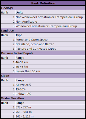

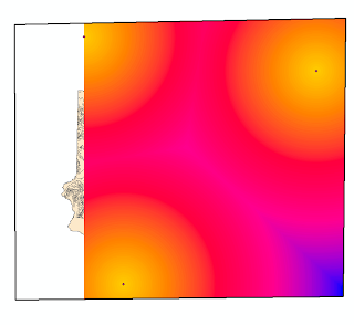
Another important factor when choosing the appropriate area to establish a sand mining is the transportation cost. Because this resource is commonly transported by railroads, it’s better for the owner to be close to the railroad terminals. Wisconsin rail depots were available and were used to run Euclidean Distance in Trempealeau County – in this matter, it’s important to remember that the real-world distance for this case shouldn’t be Euclidean, but Manhattan distance. An approach with network analysis as observed in previous exercises could be useful. Euclidean distance will be used for simplicity purposes though. As it’s important to limit the results only to the area of interest, a mask based on the county boundary would result in a distorted result, since there are no depots inside it. To go around this problem, a polygon was drawn within the closest depots and used as a mask. Because the west extent of the county exceeds the west extent of the depots, the result didn’t cover the entire county (Figure 4). A fake depot was created far west from the county – to guarantee that it wouldn’t affect the distance found by the tool – and then deleted after acquiring the appropriate results (Figure 5). The definition of ranks was based on how far the values were from the mean (41km), the range of the first Standard Deviation (10 km) resulted  on the medium rank, while the other ranks were based in what was left from this interval, always thinking – the closer, the better.


Figure 4 - Problems faced with Euclidean Distance
Figure 5 - Problem-Solving with Hypothetical Feature


A really steep area is also not appropriate for sand mining, so the calculation of slope was necessary to find the appropriate areas. For that, the DEM obtained by USGS was used to run the slope tool. Because the result was too coarse, focal statistics were used to smooth the slope values. The identification of which interval of slope was hard to be found in the literature, so a different path was taken to determine that. The Extract Values to Points tool (Figure 7) was used to obtain the slope the existing mines are located in. By analyzing the statistics, the most appropriate areas would be in the interval of the first standard deviation (5.5% - 19.2%). Therefore, values lower than 19% obtained a high rank. The interval between the first standard deviation and the second standard deviation (19.2%-26%) resulted in the medium rank; while any percentage slope higher than that would have the lower rank (Figure 6).


Figure 6 - Slope Intervals for Ranking


For last, the sand mines need to have easy access to water because this resource is essential to separate the different sizes of sand grains. Therefore, water table elevation contours were obtained from the Wisconsin Geological Survey and then converted to a raster with the Topo to Raster tool. Then, the values were categorized in three ranks based on an equal interval classification – the closer to the surface, the higher the elevation, the better for the sand mine owner.


Figure 7 - Suitability Model


After all the criteria were categorized by the Reclassify tool, the Raster Calculator tool was used to obtain the index, ranging from 1 (lowest suitability) to 15 (highest suitability). The urban and wet lands needed to be removed, so after a binary reclassification (wet and urban areas are 0 and others are 1), this raster was multiplied by the previous, resulting in a more complete index for sand mining suitability.

Impact Index

As mentioned, the second section will then study the impact of sand mining that can have three dimensions: the soil fertility where it’s located, the noise and dust that can reach urban areas, schools, rivers and airports, as well as the visibility from traditional parks and trails located in Trempealeau County. All the features for this section – with exception of the elevation model – were obtained by the official Trempealeau County Geodatabase, available online.

It’s not appropriate that the sand dust reach rivers, once that would change the environmental dynamic by the accumulation of grains. In the same way, it should not be present in densely populated areas, as schools and urban. For last, the dust could compromise airplane pilot visibility essential to landing and takeoff. Considering the 640 meters range of the noise and dust shed, for all these features, the highest risk would be in distances smaller than 640 meters, the medium would be between that and its double – 1280 meters – and then, the lowest risk would be distances higher than 1280 meters (Figure 8).

However, when deciding which features to use to apply the euclidean distance, some elements should be considered. There are a few ways to determine where are the “densely populated areas”. Although the National Land Cover Database was already downloaded, it was made for a larger area and it might be, then, generalized. Because of that, the Zoning Districts feature class obtained specifically from the county geodatabase was used. Also, for the streams, if the entire feature class was considered, no areas in the county would have low risk. Hence, it’s important to find which types would be more important, and for that, the ones with Primary Flow in Water Perennial were selected and exported as a new feature class, and this one was in fact used for the Euclidean distance. 

Figure 8 - Rank Intervals for Risk Criteria


Trempealeau County also has important statewide trails and parks, and it wouldn’t be a good think that their viewpoints would actually show a sand mine instead of a nice view. That would compromise the tourism in the area, and therefore its economy. Therefore, the application of the Viewshed Tool on the trails and parks – based on the USGS elevation – would result in two distinct classifications over the entire county: areas visible from the trails and parks, and areas not visible by them.

For last, a polygon feature class containing different types of land allowed to find where the most fertile areas were. In other words, areas where the sand mines shouldn’t be located at. The highest impact is in prime farmland or farmland considered of statewide importance. Some areas were prime land if some conditions were met, for instance, being drained and/or not flooded during growing season. Because they are only prime farmlands if those criteria are met, their risk level was considered medium. For last, areas that were not prime farmland had a low risk rank. For last, the ranked raster were added to each other using the Raster Calculator, resulting in a raster index model, ranging from 1 - lowest impact - to 21 - highest impact (Figure 9).


Figure 9 - Risk Model


Results


By the examination of the Figure 10, there are limited areas that are completely not suitable due the land use – located mainly in the south – close to the main river – as well in some areas close to the streams. Mainly, the predominance of yellow colors in the map reveals an interval between 8 and 12 in the index, which can be considered reasonable, considering the extension of these values over the county. However, there is no doubt that the northern area has more advantages when establishing a sand mine, where there are more locations with the top level – 15.

Unfortunately, the suitability model does not match that much with the risk model (Figure 11). In other words, there are limited areas with high suitability and low risk at the same time. For the impact model, the county is almost completely taken by the reddish colors referred to risk levels between 16 and 21 (the maximum). A few areas in the north are covered by greenish colors, representing low risk; which fortunately can be overlapped by the same areas of medium to high suitability in the previous model.


Figure 10 - Suitability Map


Figure 11 - Risk Analysis Map


Discussion

It’s interesting to notice the contradiction between suitability and risk. The suitability brings the interest of the companies that will establish their mines, in making it more profitable and economically encouraging. It would be easier to decrease the social and environmental risk not only for sand mining, but many industries establishments if the variables for suitability locations matched to the low-risk areas. However, as seen in the results, this is not trivial – in many cases, a low risk area is not suitable or has low suitability for the activity being proposed. Companies tend to be more driven by the economic outcomes rather than the impact they will cause in the society and environment – unless regulations require them to, being constantly enforced. The result is society and environment being frequently impacted and a high demand for the government to solve these issues – while it could have been prevented from the beginning, at the establishment of the organizations.

Regarding the data and the process, it’s important to recall that the criteria is hypothetical and should not be applied directly to a real-world specific situation – such as establishing an actual sand mine in Trempealeau County. In these cases, a detailed study should be made, going more deep on the criteria and rank intervals. The procedures in GIS, however, would remain the similar and they are the most important goal of this exercise.

This project included a number of challenges related to the use of raster. Compared to vector, this model tends to have much larger files, due to the cell size: the higher the resolution, the larger the file and the harder to use it on hardware with low performance. The same is true for vector: the higher the resolution (number of nodes in a feature), the more computer demand you’ll have. However, this problem is higher when dealing with raster. One example is the use of the viewshed tool (Figure 12): for each pixel, the tool has to take the elevation of all the pixels in between to determine the visibility. The result is a very time-demanding tool. While the tool naturally takes a long time to run, the amount of 3 hours and 26 minutes is not common, and occurred due to some issue with the server.

Figure 12 - Viewshed Tool


Some strategies to improve analysis efficiency can be applied, though. The resolution being used needs to fit the purposes of the project: although high resolutions are commonly desired, in this case they might not be the best option. If only a high resolution raster is available, resampling techniques can be used to increase the pixel size. Another strategy is to put the “Extract by Mask” tool always before all the others, in order to avoid analysis in unnecessary pixels and make sure the analysis is being made only in your area of interest.

Conclusion

Despite the challenges faced, the project was successful in using all the necessary tools to come to a complete result. The need of rethinking different techniques to go around the problems found was essential to acquire problem-solving skills and actually learn how to deal with GIS independently, especially with the use of the Arc GIS Help Desktop.

Regarding the findings, the spatial analysis offers an alternative to find areas with both high suitability and low risk. It was mentioned how hard it’s for these two variables be found together, but it’s even harder – if even possible – to find these cases without the spatial analysis. A deeper analysis of each criterion can find special areas where both variables are found, which can be used by the government to encourage sand mines to be established in that area, supporting planning initiatives.
  
Data Sources and References
MRLC. National Land Cover Database, 2006. Available on <http://www.mrlc.gov/nlcd06_leg.php> Access on April 21st.

TREMPEALEAU COUNTY. Trempealeau County Geodatabase. Available on <http://www.tremplocounty.com/landrecords/lrd_Data_Dictionary.htm> Access on April 21st.

USGS. The National Map Viewer. Available on <http://nationalmap.gov/viewer.html> Access on April 21st.

Thursday, April 4, 2013

Network Analysis: Sand Transportation Impact on the Roads.


Introduction

This exercise takes part of a bigger project analyzing the impact of sand mining in Wisconsin, in this case, dealing specifically with the road deterioration. At the moment of the county roads construction, it was not predicted a growing mining market, so they don’t necessarily have the appropriate infra-structure to support the sand transportation. Trucks loaded with sand are extremely heavy and can compromise the quality of the roads. The counties need to be aware of the cost related so they can apply the appropriate taxes to the sand mines, which will be used to road management. Therefore, the goal is to provide the cost per year for each county, related to the sand transportation.

The use of Geographic Information Systems is essential to solve this problem. Thanks to the previous exercises, the sand mines are already geocoded, consisting in a point feature class. Railroad terminals are available and are the destination for the trucks. Network Analysis provides the most likely routes taken between these features and then it’s possible to estimate the cost by county.

Methodology

Firstly, the geocoded mines need to be merged to the existing mines on the Trempealeau geodatabase. With the data prepared, it’s necessary to run the network analysis tool. There are some different options of network analysis, such as: New Route; New Service Area; New Closest Facility; New OD Cost Matrix; New Vehicle Routing Problem; and New Location-Allocation. Since first a railroad terminal needs to be assigned to each mine, and then the routes need to be applied; the New Closet Facility is the appropriate tool to be used (Figure 1).

The distance from each route can be applied to a formula to estimate the impact cost, however, the results of this tool are in time units. The feature can then be exported as a feature class, which will contain a field with the shape length. It’s extremely important to use the object-oriented model in this case, to guarantee the reliability on this field. A projected coordinate system needs to be applied to this feature class; otherwise, the shape length will be in decimal degrees – meaningless for this project.

The routes need to be divided by county so the appropriate government can deal with the road management. A summarized inside join is not appropriate because it would maintain the shape of the original route, even if it’s over the county boundary. The routes need to be clipped, but the use of the clip tool repeatedly is not a convenient way to do this. The identity tool is appropriate for this case, since it has the same idea as the clip, but works for more than one county. Multiple routes will be resulted for each county, reason why it’s then necessary to run the summarize tool. A similar result could be obtained by using the intersection tool. However, some of the routes are located outside Wisconsin and would be disregarded by this tool.

Figure 1 – Data Model for Network Analysis


The determination of the cost in dollars is going to be made using a hypothetical calculation, since the math involved in this estimative is complex and it’s not the focus of this project by now. An estimative of 50 truck trips per year and a cost of U$0.022 per mile is applied, both for loaded truck – in direction to the railroad terminal, as well as unloaded truck, in the way back. Therefore, the formula used is the distance of all the routes, per county, in miles, multiplied by 2.2 (50 truck trips * 2 ways * U$0.022).

However, since the coordinate system has meter units, first it’s necessary to create a need field and use the calculate geometry tool to provide its distance in miles. Only then the table can be exported as a .dbf file to be manipulated on Microsoft Excel in the production of graphs. Joining the cost stand-alone table to the spatial feature class for the counties is interesting to show the spatial distribution of the cost. It supports the analysis of why some counties have higher cost than others and its relation to the amount of mines and railroad terminals.

In this analysis, the use of statistical techniques such as correlation with Pearson’s I is used to test the hypothesis of a relation between the variables from the project. A null hypothesis will always state the lack of relation between the given variables, while the alternative affirms the presence of a linear relationship.

Results

Intuitively, it was expected to find higher costs in counties containing a higher number of mines. However, a primary analysis already showed that was not the case. Trempealeau is the county containing more mines in the geodatabase created – although this is due the better quality of the source, and not necessarily because the county does contain the most mines in the real-world. It was expected to find the higher cost in this county, but by looking at the resulting table (Figure 2), La Crosse appears to be the highest cost.

Figure 2 – Cost, mines and railroad terminals by county.


A graph can potentiate the examination (Figure 3), where it’s noticed that although it’s not in the first place, Trempealeau does have a high cost as well. The counties with the highest costs are La Crosse, Trempealeau, Eau Claire and Chippewa. All the other counties’ cost is lower than U$1,000 per year.

Figure 3 – Sand Transportation Impact per County


Comparing these four main counties to the amount of mines, only Trempealeau has a significant number of mines (64). La Crosse – where the highest cost is – contains only one mine; while Eau Claire and Chippewa contains 3 and 15 respectively. A map showing the cost distribution overlaid by the routes, mines and railroads terminals can elucidate the reasons for this pattern (Figure 4).

Figure 4 – Sand Mine Flow in Wisconsin and Related Cost


Although the low amount of mines in La Crosse, it contain the only railroad terminal in the within all its neighbor counties. Since Trempealeau county is at north of La Crosse, all the numerous mines located at the south of the Trempealeau will be directed to the railroad terminal in La Crosse. This only railroad terminal attends three counties (Buffalo, Trempealeau and Monroe).

The same pattern explains the high cost for Eau Claire and Chippewa: Eau Claire railroad terminal is located close to the boundary with Chippewa. Therefore, this terminal attends 10 counties besides Eau Claire and Chippewa (Burnett, Washburn, Barron, St. Croix, Dunn, Pierce, Pepin, Jackson, Trempealeau and Buffalo). Then, the counties’ roads in the way of a route from a distant mine to get to this terminal will also be compromised.

Then, it’s necessary to have a perspective of this issue not only focused on the amount of mines, but also in the presence of railroad terminals. However, this doesn’t mean that the pure existence of railroad terminal will consist in a high cost: that will only happen when there are mines around that are not served by other railroad terminals. There’s no linear relationship between railroad terminals and cost without including other variables, which can be noticed by the Pearson’s I results (Figure 5). A significance level of 0.71 fails to reject the null hypothesis, which would affirm the existence of an association between the variables.

Figure 5 – Correlation results

In the other hand, the number of mines is, indeed, statistically related to the final cost. A scatter-plot graph can illustrate better this relation (Figure 6).  As imagined, the higher the number of mines, the higher the cost. However, although the significance level of 0.00 allows the rejection of the null hypothesis with a confidence interval of 99%, the pearson coefficient of 0.56 determines only a moderate relation. Therefore, the spatial element is essential to find the inter-relations between all these variables together, instead of dealing with them isolated.

Figure 6 – Positive trend line between cost and number of mines.


Conclusion

The main goal of this project is to be able to determine how the counties should apply their taxes, which will be directed to the road management. However, if some counties that don’t even contain a mine are having their roads affected, like Washburn, the application of taxes to the county mines gets compromised. Even though the railroad terminals centralize the routes to their county, it wouldn’t make sense to charge them, since the interest of using the roads is actually in the mines.

The main problem in this scenario is the lack of railroad terminal in western Wisconsin, which makes really distant mines have to count on a few locations in La Crosse or Eau Claire. The counties should encourage, thus, encourage the creation of railroads in their own county, instead of depending on a far location. However, this is expansive and might not be economically worth, not being exactly interesting for them.

Therefore, it’s suggested that this issue don’t be restricted by the county boundaries. A state level management can be helpful to deal with the relations between the counties containing railroad terminal and the ones who doesn’t, but do have lots of mines. It would be interesting if the collection of taxes could be done accordingly to all the degradation each mine is responsible for. Then, the cost could be distributed by the counties where the routes fall on to.

However, this issue involves a complex inter-relation of agreements and laws that cannot necessarily fit the ideal scenario. The registration of mines being recently done by the government can later provide a more accurate and complete set of data, similar to the one found for Trempealeau. This would allow a more realistic answer to this issue.

Also, alternative transportation methods might be used, beyond railroads. In the same perspective, the commercial network needs to be considered: if the sand mines are providing sand to a facility in their own counties, or closer than the railroad terminal, there wouldn’t be the need to use those routes. Therefore, this project has important findings in the elements that need to be taken in consideration and encourages more study on this subject.